How to Freeze Column in Excel: A Complete Guide
When working with large datasets in Microsoft Excel, it is common to lose track of your data headers as you scroll horizontally. To prevent this, you can use the Freeze Panes feature. This allows you to keep a specific area of a worksheet visible while you scroll to another area of the worksheet, ensuring that your identifiers remain on screen at all times.
Whether you need to lock the first column for a client list or freeze multiple columns for a complex project tracker, learning how to manage your view is essential for data accuracy and efficiency.
Why You Should Freeze Columns in Excel
Freezing columns is more than just a convenience; it is a tool for data integrity. When you are analyzing hundreds of rows and columns, scrolling away from your primary identifiers (such as "Employee Name" or "Product ID") can lead to manual entry errors. By locking these columns, you maintain a constant reference point, which streamlines the process of data entry and auditing.
How to Freeze the First Column
If you only need to keep the leftmost column visible, Excel provides a one-click shortcut. Follow these steps:
- Open your Excel workbook and navigate to the sheet you wish to modify.
- Go to the View tab on the top Ribbon.
- Locate the Window group and click on Freeze Panes.
- Select Freeze First Column from the drop-down menu.
Once selected, a thin grey line will appear to the right of column A. No matter how far you scroll to the right, the first column will remain stationary.
How to Freeze Multiple Columns
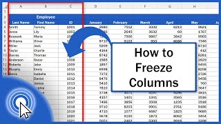
Sometimes, freezing a single column isn't enough. You may need to lock the first three or four columns to keep all your primary categories visible. To do this, you must manually define the freeze point.
To freeze multiple columns, follow this specific selection logic: select the cell that is to the right of the columns you want to freeze.
For example, if you want to freeze columns A and B, you must select cell C1. Here is the step-by-step process:
- Click on the header of the column immediately to the right of the area you want to lock (e.g., Column C).
- Navigate to the View tab.
- Click Freeze Panes.
- Select the first option in the list, also titled Freeze Panes.
By selecting the cell or column to the right, you are telling Excel that everything to the left of that selection should remain locked.
How to Freeze Both Rows and Columns Simultaneously
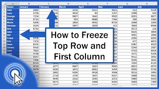
In many professional spreadsheets, you need to keep both the top header row and the first few columns visible. This is the most powerful way to use the Freeze Panes tool.
To achieve this, you must select a single cell that acts as the "anchor" for the freeze. The rule is to select the cell that is right below the row and at the right side of the columns you wish to freeze.
Example: If you want to freeze the top row (Row 1) and the first column (Column A), you should select cell B2. Then:
- Click cell B2.
- Go to the View tab.
- Click Freeze Panes and select Freeze Panes.
Now, as you scroll down, the top row stays put, and as you scroll right, the first column remains visible.
How to Unfreeze Columns
If your data structure changes or you no longer need the columns locked, you can easily revert the worksheet to its default state.