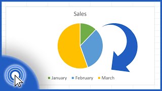
Chart With Names: How to Make Your Excel Visuals Clear and Professional
When you share data, a chart with names is often the first thing your audience notices. Properly labeled series, axes, and legends turn raw numbers into a story that can be understood at a glance. This article walks you through the essential steps for adding, renaming, and dynamically updating names in Excel charts, so every single data point speaks clearly.
Why Naming Matters in Excel Charts
Names do more than just look pretty. They improve:
- Readability – Viewers can instantly identify what each line, bar, or slice represents.
- Accuracy – Clear labels reduce the risk of misinterpretation, especially in presentations.
- Accessibility – Screen‑reader users rely on descriptive names to understand visual content.
In a business setting, well‑named charts also speed up decision‑making. For example, unlocking the power of Pivot Tables—transform your data into insights today! Watch the tutorial to see how a clean chart can complement a robust pivot analysis.
Adding and Renaming Series Names
Step‑by‑step: Insert a basic chart
- Select your data range, including column headers.
- Go to Insert ► Charts and choose the chart type you need.
- Excel automatically uses the header text as series names.
Renaming a legend entry
If the default name isn’t descriptive enough, you can rename it directly:
- Click the chart to activate the Chart Elements pane.
- Select the legend, then click the specific entry you want to change.
- Press F2 or double‑click to edit the text.
This method is demonstrated in a short video tutorial: Watch here. The video describes two different ways to rename a legend in Excel, making it easy to choose the approach that fits your workflow.
Dynamic Naming Techniques
Linking names to cells
For charts that will be updated regularly, link the series name to a cell:
- Enter the desired name in a spare cell, e.g., B1.
- In the chart, select the series, right